COMPUTING SCIENCE
AND MATHEMATICS
AND MATHEMATICS
|
COMPUTING SCIENCE
AND MATHEMATICS |
|
| Dr David Cairns Evolving Models of Collagen | |
|
Aims This EPSRC funded project aimed to develop a general method for applying Genetic Algorithms (GA) to the process of identifying the location and strength of intensity peaks in Bragg reflections in X-ray diffraction images of semi-crystalline structures such as collagen. Background The observed diffraction patterns for fibrous structures such as collagen tend to be complex with large numbers of overlapping Bragg reflections. In order to calculate the three-dimensional structure of an object using X-ray diffraction techniques, it is necessary to be able to quantify the intensities of each Bragg reflection that is produced. A diffuse background scatter is also associated with such diffraction patterns meaning useful information can be difficult to retrieve. The following image shows a recorded X-ray diffraction pattern (with background scatter removed) of type I collagen with X marks indicating candidate Bragg peaks. In order to extract structural information from the recorded data, we must identify which of these locations are actually contributing to the construction of the original image and to what degree. 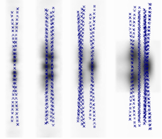 Figure 1: Recorded X-ray
diffraction image of type I collagen with X marks indicating possible locations
of Bragg reflection peaks. This image shows the 4 separate groups that are
solved in the images below.
Figure 1: Recorded X-ray
diffraction image of type I collagen with X marks indicating possible locations
of Bragg reflection peaks. This image shows the 4 separate groups that are
solved in the images below.
In order to determine where true peaks in the reflections are located (rather than an apparent peak created through the overlap of two adjacent peaks), we can place a 2-dimensional Gaussian function at candidate Bragg peak positions (the peak positions can be calculated from the known lattice structure) to build up a simulated model of the original image. We can then compare the modelled image with the observed image. Adjustments can then be made to the modelled peak intensity values in order to bring the modelled image closer to the observed image. An example of a sample (poor) placement of 2D Gaussians is shown in the following image with a comparison against the recorded data together with a difference map indicating errors. Horizontal and vertical sections through these images are also shown for further comparison. 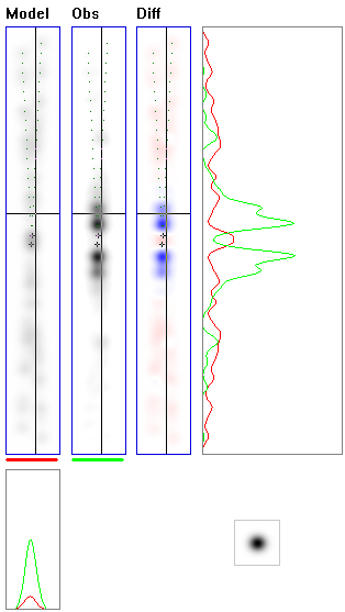 Figure 2: A poor initial solution (Model) for the recorded pattern (Obs) and a difference map between the two images (Diff). Potential locations of the Bragg reflections are shown as small points in each image and the 2D Gaussian placed at each reflection point is shown in the bottom right. The 'Model' image is a composite of these Gaussians placed at each of the points (symmetrical points in the bottom half are not shown) where each Gaussian's level of intensity is varied between 0 (not shown) and 1 (a replication of the sample 2D Gaussian in the bottom right). The task of the GA is to build the image 'Obs' by placing Gaussians at the reflection points and varying the Gaussian strength. A vertical and horizontal cross section of the Model (red) and Observed (green) is also shown indicating the difference between the two images at the given points in the cross sections. The goal of this project was to develop a methodology using Genetic Algorithms that would identify the peaks that correspond to a given image and also calculate the relative contribution to the overall image. In order to evaluate the effectiveness of the approach, solutions were generated and compared against the original diffraction data and the resultant difference map was analysed for discrepancies. The GA approach repeatedly generates new solutions to a problem from a population of previous solutions, starting from an initial random set. The example above shows one potential solution in the population. Typically there will be on the order of 50 solutions in the population with some solutions having a better fit than others. Each new solution tends to be generated from relatively high scoring individual solutions in the previous generation (in this case, the best score is 0, indicating no difference between source and model) and �inherits� the positive traits from the parents used to derive it. In order to use a GA with a new problem, three elements must be implemented:
In this study, the parameter set used to define a possible solution was defined by the set of Gaussian intensity values assigned to each of the potential Bragg reflection co-ordinates (the X marks in the first image). A value of 0 assigned to a particular co-ordinate indicated that no reflection was centred at this point and a value of 1 indicated a 2D Gaussian at full intensity should be placed at the given co-ordinate. Values between these limits reduced the strength of the Gaussian that was placed at a given co-ordinate. The goal of the GA was therefore to find the optimal set of intensity values that would best recreate the recorded image using only these points and placements of 2D Gaussians. Generation of a solution from a parameter set involved placing 2D Gaussians at the co-ordinates that had values greater than 0 such that a composite image was created by summing all the Gaussians specified by the solution (the 'Model' image shown in Figure 1). The fitness of this solution was evaluated by using a form of n space Euclidean distance measure between the observed image and the modelled image where n is the product of the horizontal and vertical dimensions of the recorded image ('Score' in Figure 1). High scoring solutions have values close to 0 indicating minimal difference between them and the source image. In order to generate a new solution to add to the population, the following procedure is applied:
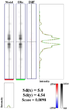
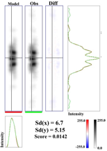
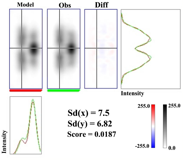
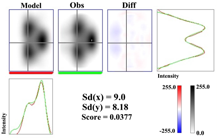
Since the two parent solutions tend to have a relatively high level of fit in the population, their combined parameter values usually create a new solution that also has a good level of fit. The use of mutation and the fact that parent solutions do not always have the best fit occasionally generates a novel solution that also has a good fit to the target. These solutions would not have been reached by the more incremental crossover approach, thus overcoming issues of the population getting caught in local minima. The GA is normally left to run until the solutions it is producing have stabilised (i.e. there is no overall improvement in the population score). Depending upon the complexity of the task, this took between 10 minutes for the simpler images with relatively few closely located lattice points and 14 hours on the more complex images which had many closely neighbouring lattice points (all solutions were generated on a dedicated 3GHz Dual Xeon PC). In order to check the validity of the approach across different task, 12 different diffraction images were processed (4 groups extracted from a native, gold and iodine labelled source images). The results of using this approach are shown below for the 4 groups extracted from the native image. Each image is in the same format as shown in Figure 1 where a Model, an Observed and a Difference image is provided together with a vertical and horizontal cross section. For each cross-section a green (Observed) and red (Modelled) trace is provided which shows the intensity in each of the respective images at a given point in the cross-section. It should be noted that these lines overlap very closely, indicating a very good fit between the modelled and observed image.
It can be seen from these results that the GA approach produces a very good level of fit to the source data with only small discrepancies between the source image and the model. Given that the GA approach generates a range of solutions which can have different outcomes, we have repeated this process 100 times for each pattern and examined the variation in intensity assigned to each lattice point. The solutions have been found to be broadly stable with only small variations where points are located with 2-3 pixels of each other.
|
|